Analyzing Return Times II - Concurrent

This time we’ll discuss the concurrent model for aggregrating search results. In this post, we’re going to look at how to:

• aggregate the results concurrently
• model the algorithm run time as a random variable
• find and evaluate the CDF of our model for a couple values

This is part 2 in a series of posts that analyzes the return times of various randomized algorithms presented in a talk by Rob Pike.

If you have not read the first post, I would encourage you to start there.

Recap

Last time we analyzed the sequential method of gathering our results. We wanted to know what percent of users would recieve their results in less than 1.5 seconds. After finding the PDF of the response time, we discovered that we could only expect half of users to hit our benchmark! The experimental results were even worse due to overhead in appending the results - only 46.0% make it.

Concurrency and parallelism

How can we do better?

Well, our algorithm is just waiting for a response most of the time. If we launched all our searches and let them run at the same time, we would only wait as long as the longest search. Running these searches simultaneously is called parallel computing.

Furthermore, getting the proper results does not matter when or in what order we get them. This means our algorithm can be designed concurrently.

It is worth noting that concurrency and parallelism are not the same thing. These are often confused - so much so that Rob Pike has presented another talk on this very issue.

• Parallelism is the simultaneous excecution of two or more processes
• Concurrency is the property of an algorithm that allows it to be decomposed into multiple processes whose order of execution does not affect the correctness of the result

Because our search is not actually being offloaded to other servers, it is not necessarily parallel (though it may be if you run it on a multi-core system!)

fakeSearch is, however, sleeping most of the time. This means it will not block CPU execution and, for all practical purposes, seem to run in parallel with other fakeSearches.

GoogleConcurrent

Now we get to the algorithm.

 1func GoogleConcurrent(query string) (results []Result) {
 2  c := make(chan Result)
 3  go func() { c <- Web(query) }()
 4  go func() { c <- Image(query) }()
 5  go func() { c <- Video(query) }()
 6
 7  for i := 0; i < 3; i++ {
 8    result := <-c
 9    results = append(results, result)
10  }
11  return
12}

The keyword chan denotes a channel in Go.

2  c := make(chan Result)

Channels are pipes that allow you to send and recieve values between various threads of execution. Arrows pointing towards the channel, c <- foo, indicates the channel will be given a value. Arrows pointing away from the channel, foo := <-c, indicates a value should be recieved from the channel.

The go keyword starts a new goroutine.

3  go func() { c <- Web(query) }()

Goroutines are lightweight threads managed by the Go runtime. They are especially useful because it is practical to have hundreds of thousands running concurrently.

Here we are using go to start an anonymous function that populates the channel with the search query result.

Goroutines and channels are especially useful because they make it easy to aggregrate results without locks, condition variables, or difficult to follow callbacks. Even though this function starts several threads of execution, we can still read it more or less sequentially.

GoogleConcurrent as a random variable

In the sequential model, we had to wait for the first result then start the next search. This time we run all of them at the same time, meaning the total time we have to wait is the time the longest query takes to finish. Let’s model this as a random variable

$$ Y_{concurrent} = \text{max}(X_1, X_2, X_3) $$

Where \(X_i\) is the time to complete a fakeSearch, which we modeled as a uniformly distributed random variable in the previous post.

Cumulative Distribution Function (CDF)

With the sequential method, we wanted to see the probability that a user would wait no more than 1.5 seconds. To do this we calculated the integral of the PDF, \( f_Y(y) \), from \( -\infty \) to 1.5. This is also known as the Cumulative Distribution Function (CDF), \( F_Y(y) \), at \( y = 1.5 \)

The relation between the probability of our event, the CDF, and the PDF is written like this:

$$ P(Y \leq y) = F_Y(y) = \int _{-\infty}^y f_Y(t) dt $$

Each term is read like such

• the probability Y is less than or equal to y, which is equal to
• the CDF of Y at y, which is equal to
• the integral of the PDF of Y from negative infinity to y

CDF of GoogleConcurrent

Now let’s find the probability that users wait no more than y seconds for the GoogleConcurrent algorithm.

$$ \begin{align} F_Y(y) & = P(Y \leq y) \\\ \\\ & = P(\text{max}(X_1, X_2, X_3) \leq y) \end{align} $$

If y is greater than the largest X, it must also be greater than all X. Making this substitution allows us to decompose the problem further.

$$ \begin{align} P(\text{max}(X_1, X_2, X_3) \leq y) & = P(X_1 \leq y \cap X_2 \leq y \cap X_3 \leq y) \\\ \\\ & = P\left(\bigcap _{i=1}^3 X_i \leq y\right) \end{align} $$

The intersection, \(\cap\), of events means that each event must happen for the whole condition to succeed.

Furthermore, each fakeSearch is independent, i.e. the time taken for one search does not affect the time taken for the other search.¹ This special property implies the probability of all events happening is equal to the product of the probability of each event.

$$ \begin{align} P\left(\bigcap _{i=1}^3 X_i \leq y\right) & = P(X_1 \leq y)P(X_2 \leq y)P(X_3 \leq y) \\\ \\\ & = \prod _{i=1}^3P(X_i \leq y) = F_X(y)^3 \end{align} $$

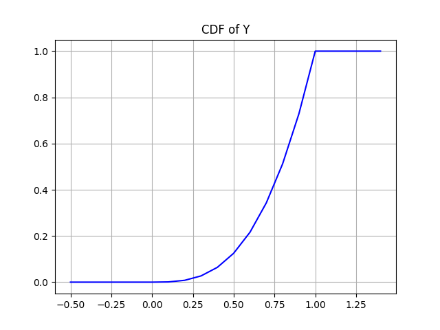
The rather satisfying result is the CDF of GoogleConcurrent simply equals the CDF of the uniform distribution cubed.

$$ F_Y(y) = \begin{cases} 0, & x < 0 \\\ x^3, & 0 < x < 1 \\\ 1, & x \geq 1 \\\ \end{cases} $$

Here’s a graph of the result

How does it compare?

With sequential, we got results back in 1.5 seconds or less 50% of the time here we get…

$$ F_Y(1.5) = 1 $$

With GoogleConcurrent we can expect to get 100% of results back in under 1.5 seconds! Of course this makes sense: no one query takes longer than 1 second and we’re running all of them at the same time.

But how fast can we get? Let’s evaluate the probability that GoogleConcurrent will finish before a few more time points: $$ \begin{align} F_Y(0.5) &= 0.125 \\\ F_Y(0.8) &= 0.512 \\\ F_Y(0.9) &= 0.729 \\\ \end{align} $$

Reading the second line, we can expect 51.2% of requests to be processed in 0.8 seconds or less

Running an experiment with 2000 samples, 49.5% of requests were processed in 0.8 seconds. Once again the experimental results were slightly slower than the theoretical results - presumably due to overhead.

In addition to the outstanding speed benefits we get from running the searches in parallel, we also give ourselves some room to expand. In the previous case, adding each additional search would increase the limit of our potential wait times by 1 second. With GoogleConcurrent even though our expected wait time will get closer and closer to 1 second with each additional search, our max wait time will never exceed that 1 second bound!²

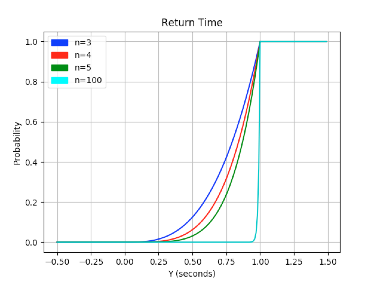
The graph above shows us the CDF of Y as the number of different searches, \(n\), increases.

What next?

Running the search in parallel significantly reduced our expected wait times. Can we do better? Until seeing Rob’s talk, I didn’t know how, but next post we’ll look at how using replicated services will allow us to improve even more!