Analyzing Return Times III - Replicated

This time we’ll discuss the replicated model for aggregrating search results. We’re going to look at how to:

• fetch the first result from replicated services
• model the algorithm as a random variable
• compare the replicated method against the concurrent method

This is part 3 in a series of posts that analyzes the return times of various randomized algorithms presented in a talk by Rob Pike.

If you have not read the first post, I would encourage you to start there.

1. Sequential
2. Concurrent

Recap

Last time we analyzed the concurrent method of gathering our results. We ran all our searches at the same time and aggregated the results such that we only had to wait as long as the longest request.

We discussed the CDF of a random variable and how it’s found. Using the CDF of the return time for a GoogleConcurrent call, we compared it against the sequential method. We found it was much faster and could expect over 50% of responses to take less than 0.8 seconds.

Replicated services

With replicated services, we’re creating multiple copies of each service to do the same work. At first glance, it may seem like a waste to duplicate our efforts but, due to the random nature of our services, it can improve our expected return times. The basic idea is that the more copies of the service call we make, the more likely one of them will return relatively early.

Getting the first result

We’re going to need a fuction that gets the first result from a set of replicated services.

1func First(query string, replicas ...Search) Result {
2  c := make(chan Result)
3  searchReplica := func(i int) { c <- replicas[i](query) }
4  for i := range replicas {
5    go searchReplica(i)
6  }
7  return <-c
8}

Let’s describe this in more detail.

The elipsis in the function parameters, ...Search, denotes a variadic parameter. It allows us to pass any number of arguments in the parameters. In our case, that’s an indefinite number of search replicas.

  searchReplica := func(i int) { c <- replicas[i](query) }
  for i := range replicas {
    go searchReplica(i)
  }

Above, we define a function, searchReplica, which populates a channel with the results from a replica specified by its index. After that, we loop through all the replicas starting a goroutine for each.

  return <-c

Finally, we return the result that first appears on the channel.

First as a random variable

As opposed to GoogleConcurrent, which aims to find the max wait time, First tries to find the minimum wait time. Modeling this as a random variable \(Z\), we get:

$$ Z = \text{min}(X_1, X_2, X_3) $$

Where \(X_i\) is the time to complete a fakeSearch, which we modeled as a uniformly distributed random variable in the previous posts.

Complementary CDF (cCDF)

Sometimes, it’s useful to evaluate the complement of the CDF - that is, the probability a random variable is larger than a certain value.

Because it’s certain some event must occur, integrating the CDF over the entire sample space always equals one. This allows us to define the complementary CDF (cCDF) as one minus the CDF.

$$ \begin{align} P(Z \leq \infty) & = \int _{-\infty}^{\infty} f_Z(t) dt = 1 \\\ \\\ P(Z > z) & = 1 - \int _{-\infty}^z f_Z(t) dt \end{align} $$

This property will soon come in handy for evaluating the CDF of First.

CDF of First

Now let’s find the probability that First will return a result in at most \(z\) seconds. We’re looking for the first fakeSearch to return from a set of \(m\) replicas

$$ \begin{align} F_Z(z) & = P(Z \leq z) \\\ \\\ & = P(\text{min}(X_1, X_2, …, X_m) \leq z) \end{align} $$

Last time, we were able to decompose the max easily because if y was less or equal to the max than it must be less or equal to all X. The same cannot be said for the min - that means it’s not so straightforward this time.

We can, however, use the cCDF to our advantage.

$$ \begin{align} 1 - F_Z(z) & = P(Z > z) \tag{1}\label{1} \\\ \\\ & = P(\text{min}(X_1, X_2, …, X_m) > z) \end{align} $$

Now that we’re making a greater than comparison with \(z\), we can split the random variables up. If the min fakeSearch takes more than \(z\) time, than all fakeSearchs take more than \(z\) time.

$$ \begin{align} P(\text{min}(X_1, X_2, …, X_m) > z) & = P(X_1 > z \cap X_2 > z \cap … X_m > z) \\\ \\\ & = P\left(\bigcap _{i=1}^m X_i > z\right) \end{align} $$

Like last time, we can make use of independence to further simplify our problem. Except now each term corresponds to the cCDF of X.

$$ \begin{align} P\left(\bigcap _{i=1}^m X_i > z\right)& = \prod _{i=1}^mP(X_i > z) = (1 - F_X(z))^m \end{align} $$

Rearranging our formula from \ref{1}, we can express the CDF of First like so:

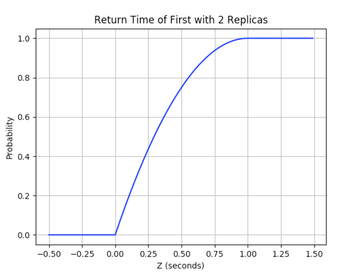
$$ \begin{align} F_Z(z) & = 1 - P(Z > z) \\\ & = 1 - (1 - F_X(z))^m \\\ & = \begin{cases} 0, & z < 0 \\\ 1 - (1 - z)^m, & 0 < z < 1 \\\ 1, & z \geq 1 \\\ \end{cases} \end{align} $$

Here’s a graph of the result with 2 replicas

GoogleReplicated

We still have to aggregate the results from each search provided from First. This looks very similar to how it was handled with GoogleConcurrent.

func GoogleReplicated(query string) (results []Result) {
  c := make(chan Result)
  go func() { c <- First(query, Web1, Web2, Web3) }()
  go func() { c <- First(query, Image1, Image2, Image3) }()
  go func() { c <- First(query, Video1, Video2, Video3) }()
  for i := 0; i < 3; i++ {
    result := <-c
    results = append(results, result)
  }
  return
}

The only major difference is we replicate each service 3 times and call First instead of fakeSeach.

Using our work from previous posts, it’s pretty easy to find the CDF of GoogleReplicated. If we model the time it takes to complete a GoogleReplicated call as the random variable \(Y\), we get:

$$ \begin{align} F_Y(y) & = F_Z(y)^n \\\ & = (1 - (1 - F_X(y))^m)^n \\\ & = \begin{cases} 0, & y < 0 \\\ (1 - (1 - y)^m)^n, & 0 < y < 1 \\\ 1, & y \geq 1 \\\ \end{cases} \end{align} $$

How does it compare?

The basic parallel method got us results back in 0.8 seconds or less roughly 50% of the time. Our improvement should now come from the fact that the more replicas we add, the more likely it is one of the replicas will respond very quickly.

For our comparison, let’s create only 2 replicas for each service (and we’ll keep the number of searches fixed at 3). Let’s see what percent we can expect to reply in 0.8 seconds or less with our improvement.

$$ F_Y(n=3, m=2; 0.8) \approx 0.885 $$

Whoah! That’s a pretty big improvement with only 2 replicas. Almost 90% of users will see the same speeds that only 50% saw without replicas.

Running an experiment with 2000 samples, 87.4% of requests were processed in 0.8 seconds.

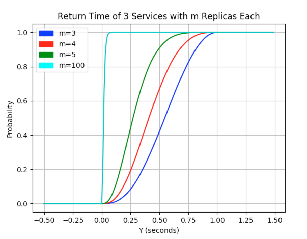
The cool thing about this method is we can move the expected return time arbitrarily close to 0 seconds.¹ Here’s a graph showing the CDF of wait times for GoogleReplicated for different numbers of replicas, \(m\)

Conclusions

So we should use replicated services in all our software, right? Well not quite.

First of all, a uniform distribution is unlikely to reflect the latency in most services. As I mentioned previously, it’s more likely services would look like a log normal distribution. Depending on your return time distribution, replicating your services could have a very small impact.

Next, it may not be worth it. Faster is (almost) always better but there’s a good chance those replicated services won’t come free. You may be able to distribute your system properly such that underutilized resources will take on this replication overhead but duplicating at this scale will probably require more resources than those that are lying idle.

One really nice use of replicated services is in maitenance and upgrades. In the two previous methods if we needed to do changes to one of the services, our entire system would have to come down. Under the new model, we can spin up new updated services then slowly remove old ones from production without degradation to the user experience.

The End

Hopefully, this series has highlighted features in Go that make building concurrent programs easier. Furthermore, I hope it’s now easier to model your algorithms as random variables and make accurate predictions about their behaviours.

Thanks for reading!